Prerequisites
Required Lablink resources
The following Lablink resources are required:
Configuration Server: config-0.0.1-jar-with-dependencies.jar
Datapoint Bridge: dpbridge-0.0.1-jar-with-dependencies.jar
Lablink Plotter: plotter-0.0.1-jar-with-dependencies
When building from source, the corresponding JAR files will be copied to directory target/dependency.
Starting the configuration server
Start the configuration server by executing script run_config.cmd in subdirectory examples/0_config. This will make the content of database file test-config.db available via http://localhost:10101.
Note
Once the server is running, you can view the available configurations in a web browser via http://localhost:10101.
See also
A convenient tool for viewing the content of the database file (and editing it for experimenting with the examples) is DB Browser for SQLite.
MQTT broker
An MQTT broker is required for running the example, for instance Eclipse Mosquitto or EMQ.
Example 1: Fixed interval data source
This example reads CSV data from the configuration server (the data can be viewed here when the configuration server is running locally). The data from the columns of the CSV source (called test1.val1, test2.val2, test3.val3, test4.n) are sent one after the other as individual measurements to a plotter. The time between two consecutive measurements is constant (set to 1 second in this example).
The CSV data looks like this:
test1.val1,test2.val2,test3.val3,test4.n
0.0,86.6,-86.6,0
40.7,58.8,-99.5,1
74.3,20.8,-95.1,2
95.1,-20.8,-74.3,3
99.5,-58.8,-40.7,4
86.6,-86.6,0.0,5
58.8,-99.5,40.7,6
...
When sent to the plotter, the CSV client’s output looks like this:
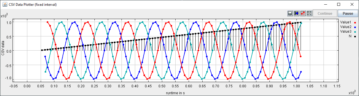
All relevant scripts can be found in subdirectory examples/1_fixed_interval. To run the example, execute all scripts either in separate command prompt windows or by double-clicking:
csv-fixed-interval.cmd: runs the CSV client, which will send data to the plotter
dpb.cmd: runs the data point bridge service, connecting the CSV client and the plotter
plot.cmd: runs the plotter, which will plot incoming data to the screen
Note
The scripts can be started in arbitrary order.
Example 2: Timed data source
This example reads CSV data from the configuration server (the data can be viewed here when the configuration server is running locally). The data from the CSV source uses a dedicated format (see here), providing data values associated to timestamps, which are sent one-by-one as individual measurements to a plotter. The timing of the measurements is determined by the associated timestamps.
The CSV data looks like this:
Device;Datapoint;Timestamp;Measurement
test1;val1;1609412400274;11,4
test1;val1;1609412401735;66,4
test1;val1;1609412402268;81,3
test1;val1;1609412403672;99,9
test1;val1;1609412404090;99,0
test1;val1;1609412405897;62,2
test1;val1;1609412406240;50,4
...
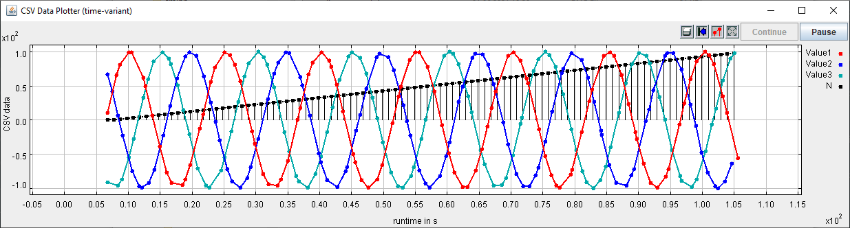
When sent to the plotter, the CSV client’s output looks like this:
Note
The plotted results from both examples may look very similar at first glance. However, if you take a closer look you will notice that in the 2nd example the measurements are not received at a fixed rate. This difference becomes obvious when you run the examples and watch the measurements being plotted in real time.
All relevant scripts can be found in subdirectory examples/2_time_variant. To run the example, execute all scripts either in separate command prompt windows or by double-clicking:
csv-time-variant.cmd: runs the CSV client, which will send data to the plotter
dpb.cmd: runs the data point bridge service, connecting the CSV client and the plotter
plot.cmd: runs the plotter, which will plot incoming data to the screen
Note
The scripts can be started in arbitrary order.