Prerequisites¶

Required Lablink resources¶

The following Lablink resources are required for running the examples:

Configuration Server: config-0.0.1-jar-with-dependencies.jar
Datapoint Bridge: dpbridge-0.0.1-jar-with-dependencies.jar
Lablink Plotter: plotter-0.0.1-jar-with-dependencies

When building from source, the corresponding JAR files will be copied to directory target/dependency.

Note

You also need a local copy of the FMU file zigzag.fmu. In case you have checked out a local copy of the lablink-fmusim repository, you can find it in the local subdirectory src/test/resources.

Starting the configuration server¶

Start the configuration server by executing script run_config.cmd in subdirectory examples/0_config. This will make the content of database file test-config.db available via http://localhost:10101.

Note

Once the server is running, you can view the available configurations in a web browser via http://localhost:10101.

MQTT broker¶

An MQTT broker is required for running the example, for instance Eclipse Mosquitto or EMQ.

Example 1: Dynamic simulation using an FMU for Model Exchange¶

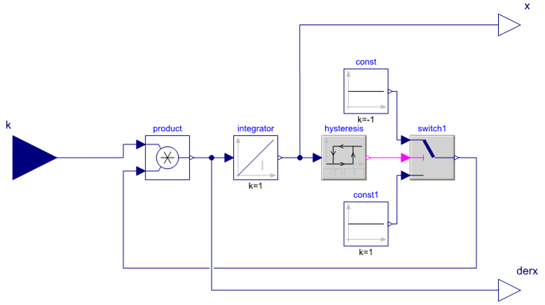
The figure below shows the graphical representation of the zigzag model used in this example. It comprises an integrator, whose input is a constant (model input variable k), and a hysteresis controller, which switches the sign of k in case the integrator’s output variable x crosses a certain threshold (low: -1, high: 1). The resulting output is a zigzag pattern (hence the model name). The model has been compiled with Dymola into an FMU for Model Exchange, which can be found in subdirectory src/test/resources.

To run the example, edit attribute FMU.URI in the FMU simulator client configuration ait.test.fmusim.dynamic_me.fmu.config to match the absolut path of the FMU file (located in your local subdirectory src/test/resources). Use for instance DB Browser for SQLite to edit the configuration.

All relevant scripts can be found in subdirectory examples/1_dynamic_me. To run the example, execute all scripts either in separate command prompt windows or by double-clicking:

fmusim.cmd: runs the FMU simulator
dpb.cmd: runs the datapoint bridge service, connecting the FMU simulator and the plotter
plot.cmd: runs the plotter, which will plot incoming data

Note

The order in which the scripts are started is arbitrary.

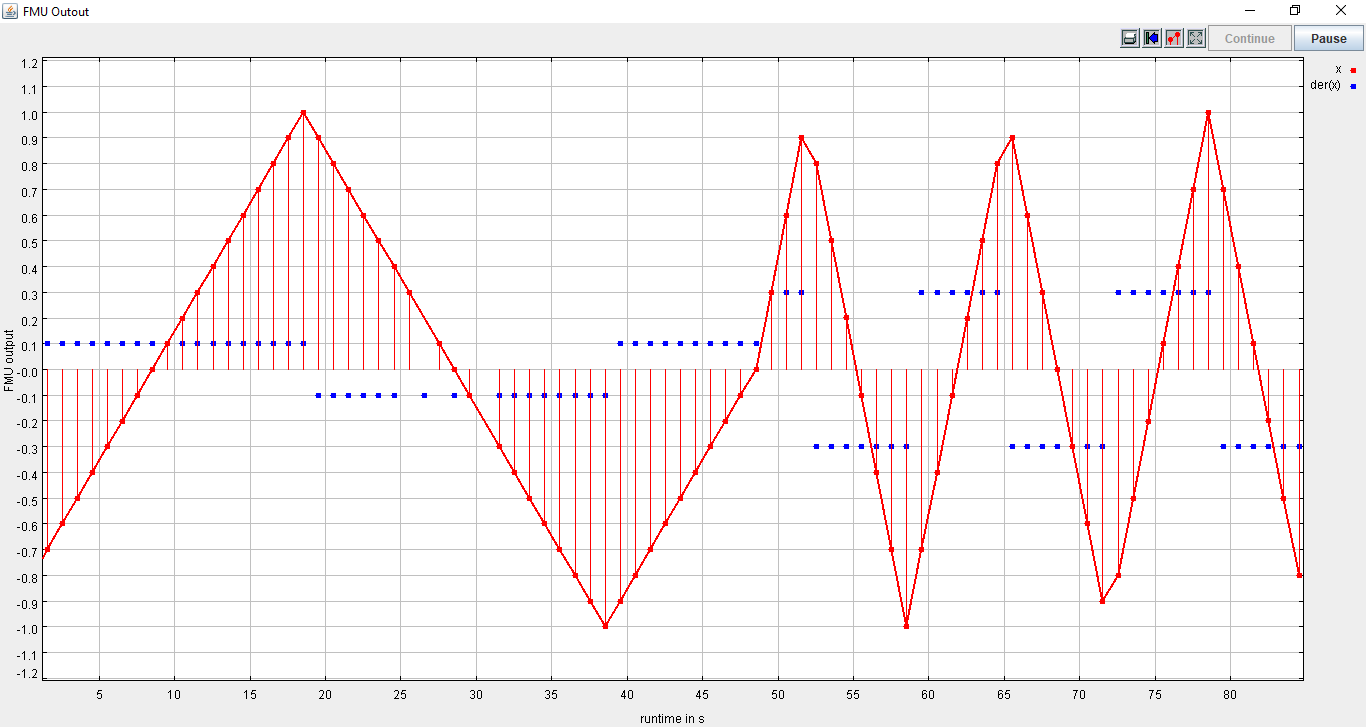
Once the FMU simulator client starts up, the client shell can be used to interact with the FMU model. For instance, input variable k of the FMU model can be changed:

llclient> svd k .3
Success
llclient> svd k 3
Success

An example of how the FMU reacts on these inputs can be seen in the following figure.

Example 2: Fixed-step simulation using an FMU for Model Exchange¶

This example uses the same zigzag model as the previous example.

To run the example, edit attribute FMU.URI in the FMU simulator client configuration ait.test.fmusim.fixedstep_me.fmu.config to match the absolut path of the FMU file (located in your local subdirectory src/test/resources). Use for instance DB Browser for SQLite to edit the configuration.

All relevant scripts can be found in subdirectory examples/2_fixedstep_me. To run the example, execute all scripts either in separate command prompt windows or by double-clicking:

fmusim.cmd: runs the FMU simulator
dpb.cmd: runs the data point bridge service, connecting the FMU simulator and the plotter
plot.cmd: runs the plotter, which will plot incoming data

Note

The order in which the scripts are started is arbitrary.

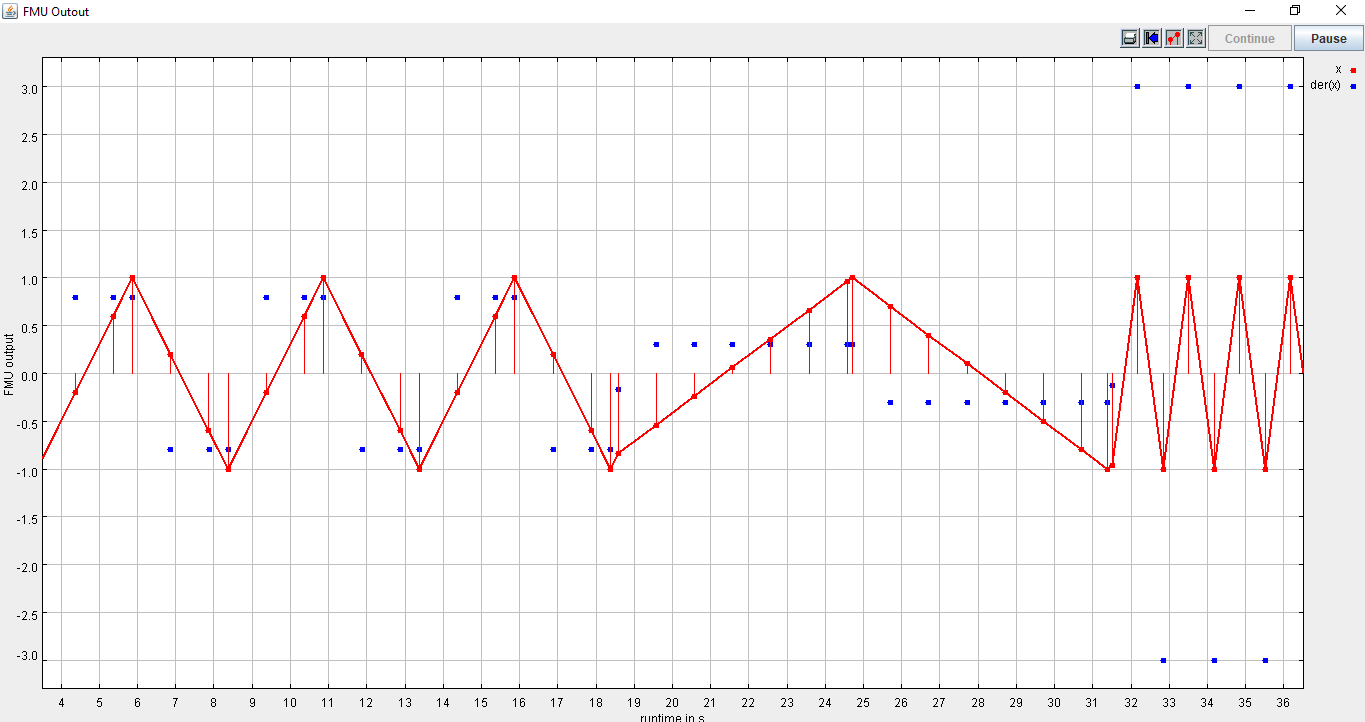
Once the FMU simulator client starts up, the client shell can be used to interact with the FMU model. For instance, input variable k of the FMU model can be changed:

llclient> svd k 0.3
Success

An example of how the FMU reacts on these inputs can be seen in the following figure. Notice the differences to the previous example, where the FMU simulator did update the outputs not only at strictly periodic intervals.